A*

Article Goal

Explain in the most straightforward way how A*’s Algorithm works. Diagrams included!

What is A*?

A* is a pathfinding algorithm that uses heuristics to guide its search. Unlike Dijkstra’s algorithm, which explores in all directions equally, A* attempts to guess the best path. It maintains a balance between:

1. The actual distance traveled from the start (g-cost)
2. The estimated distance to the goal (h-cost)

The combination of these costs $\text{f(n)} = \text{g(n)} + \text{h(n)}$ helps A* make “intelligent” decisions about which paths to explore first.

Core Components

1. Cost Functions

• g(n): The actual cost from the start node to the current node
• h(n): The estimated cost from the current node to the goal (heuristic)
• f(n): The total estimated cost of the path through node n (f(n) = g(n) + h(n))

2. The Heuristic Function

The heuristic function h(n) is what makes A* special. Common heuristics include:

• Manhattan Distance: abs(x1 - x2) + abs(y1 - y2)
• Euclidean Distance: √((x1 - x2)² + (y1 - y2)²)
• Diagonal Distance: max(abs(x1 - x2), abs(y1 - y2))

Algorithm

1. Initialization
   • Set the distance to the origin node, $g[\text{origin}] = 0$.
   • Set the distance to all other nodes, $g[v] = \infty$ for $v \neq \text{origin}$.
   • Calculate the heuristic $h[v]$ for all nodes (estimated distance to goal).
   • Set $f[v] = g[v] + h[v]$ for all nodes.
   • Add origin node to the open set (priority queue ordered by $f$ values).
   • Initialize closed set as empty.
   • Set the parent of each node to None.
2. Select Node
   • While the open set is not empty:
     • Pick the node $u$ from the open set with the smallest $f[u]$ value.
     • Remove $u$ from the open set and add it to the closed set.
3. Check Goal
   • If $u$ is the goal node:
     • Reconstruct and return the path using parent pointers.
4. Update Neighbors
   • For each neighbor $v$ of $u$ that is not in the closed set:
     • Calculate the tentative distance: $g_{\text{tentative}} = g[u] + w(u, v)$.
     • If $v$ is not in the open set or $g_{\text{tentative}} < g[v]$:
       • Update $g[v] = g_{\text{tentative}}$.
       • Update $f[v] = g[v] + h[v]$.
       • Set the parent of $v$ to $u$.
       • Add $v$ to the open set (if not already present).
5. Repeat
   • Repeat steps 2–4 until the goal is found or the open set is empty.

The shortest path is reconstructed by tracing the parent pointers from the goal vertex back to the source vertex.

Performance

Correctness

A* is guaranteed to find the optimal path when the heuristic function $h(v)$ is admissible (never overestimates the true distance to the goal).

Complexity

• Time: $O(E log V)$ using a binary heap, or $O(b^d)$ where $b$ is branching factor and $d$ is solution depth\
• Space: $O(V)$

Simple Example

Let’s walk through a simple example to see how A* works step by step. We’ll use a graph with 7 vertices (A through G) where A is our start vertex and B is our goal vertex.

Step 1: Initial Graph

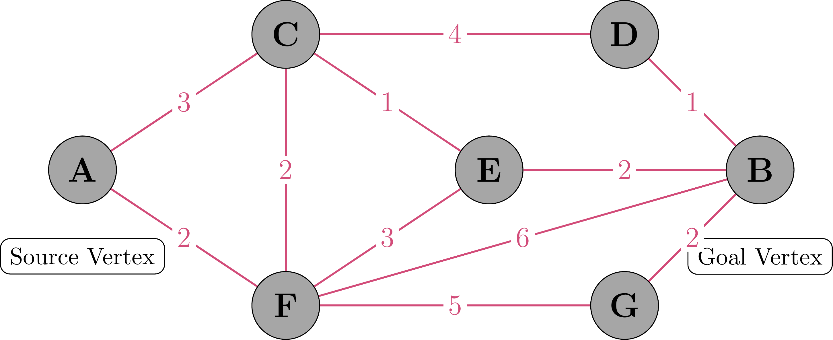
This shows our initial graph with all vertices and edges. The numbers on the edges represent the actual costs between vertices.

Step 2: Algorithm Initialization

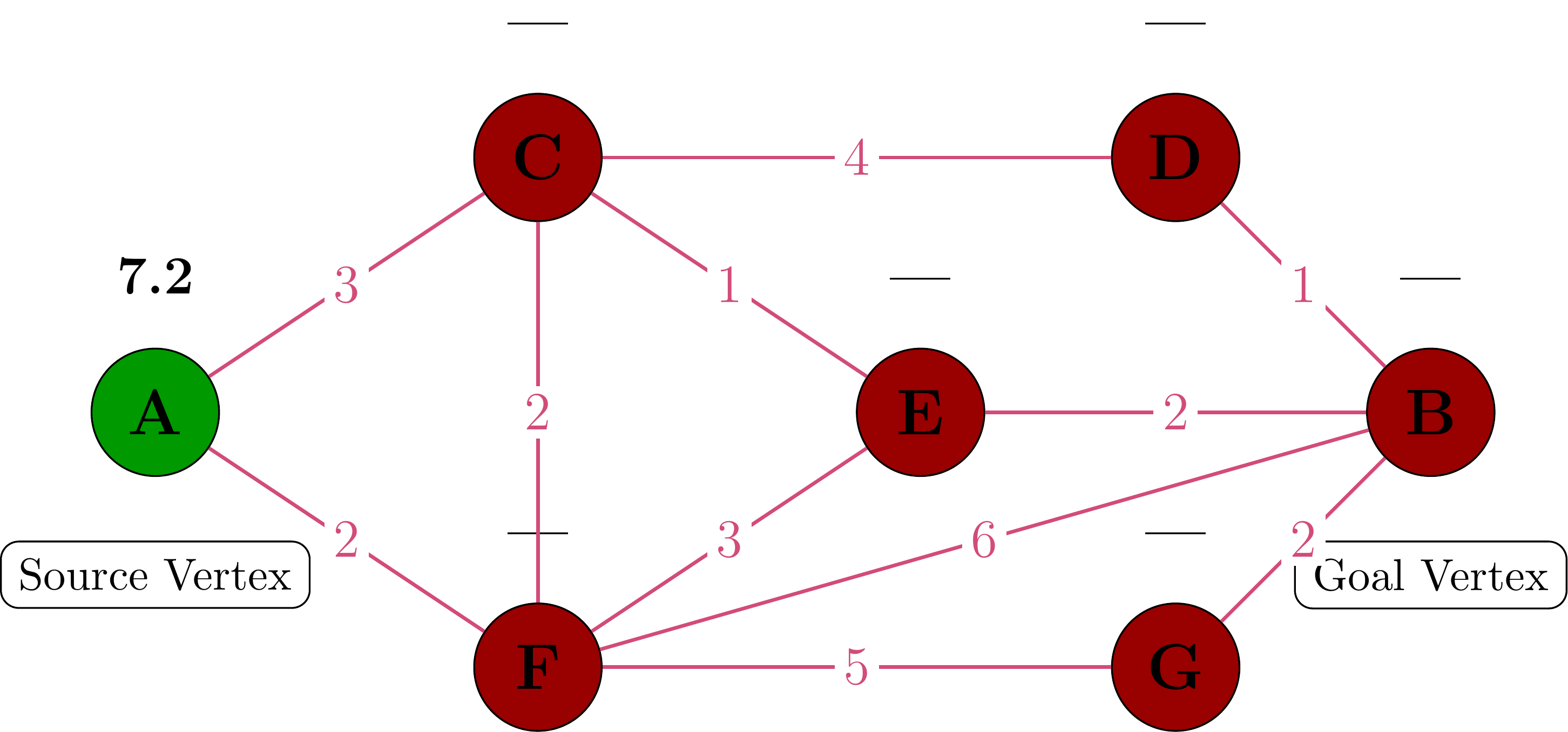
We start by:

• Setting g(A) = 0 (distance from start to start is 0)
• Setting g(v) = ∞ for all other vertices
• Calculating heuristic values h(v) for all vertices
  • h(A)=7.2, h(B)=0, h(C)=5.4, h(D)=2.2, h(E)=3.6, h(F)=6.3, h(G)=2.8
• Calculate f(A) = 0 + 7.2 = 7.2
• Adding A to the open set

Step 3: Processing Vertex A

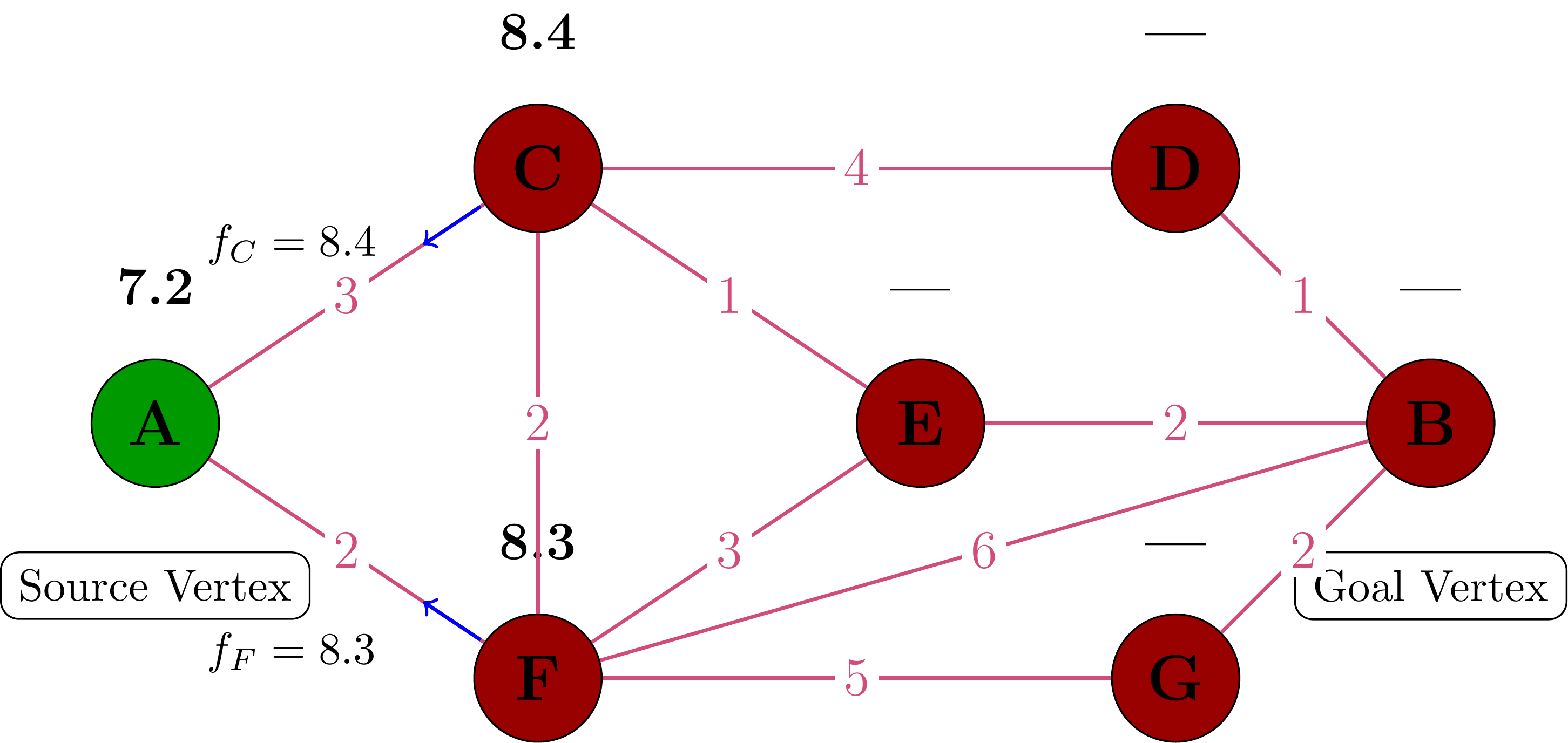
We process vertex A (the only vertex in our open set):

• Add A to the closed set (green)
• Update neighbors C and F with new g-values
• Calculate new f-values:
  • f(C) = g(C) + h(C) = 3 + 5.4 = 8.4
  • f(F) = g(F) + h(F) = 2 + 6.3 = 8.3
• Add C and F to the open set

Step 4: Processing Vertex F

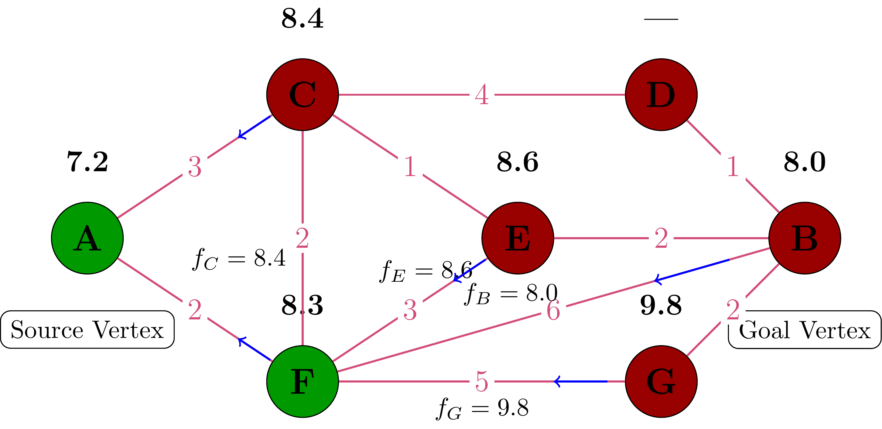
Vertex F has the lowest f-value (8.3), so we process it:

• Add F to the closed set (green)
• Update neighbors E and B with new g-values
• Calculate new f-values for E, B, G, C
  • If calculated f(C) is < original f(C), update it to the new value. It is also 8.4 so we don’t update
• Add E, B, G to the open set

Step 5: Finding Vertex B (First Time)

Goal Node is found but algorithm continues to determine optimality

Step 6: Processing Vertex C

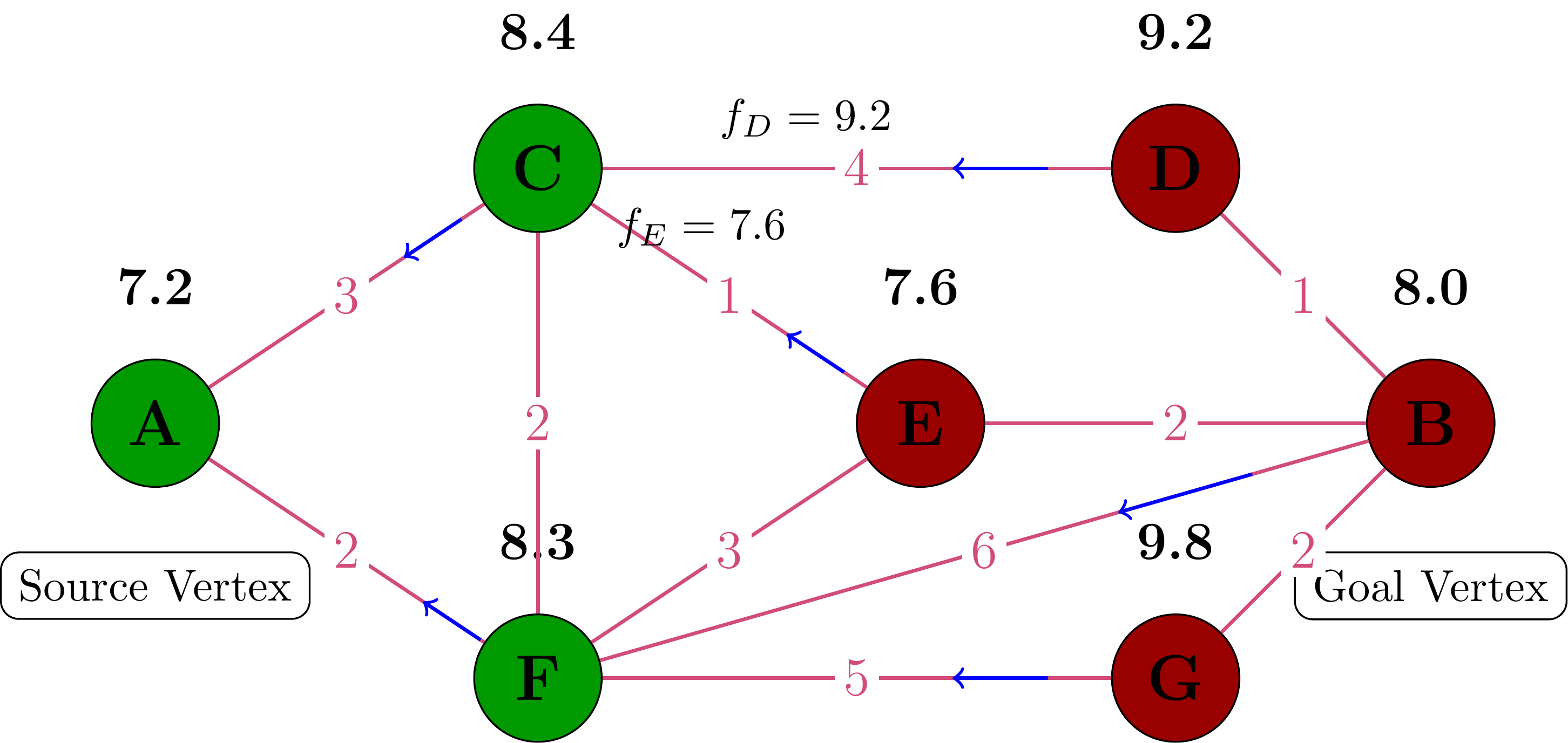
Vertex C has the lowest f-value, so we process it:

• Add C to the closed set (green)
• Update neighbors D and E with new g-values
• Note that we found a path to B with f-value = 8.0

Step 7: Processing Vertex E

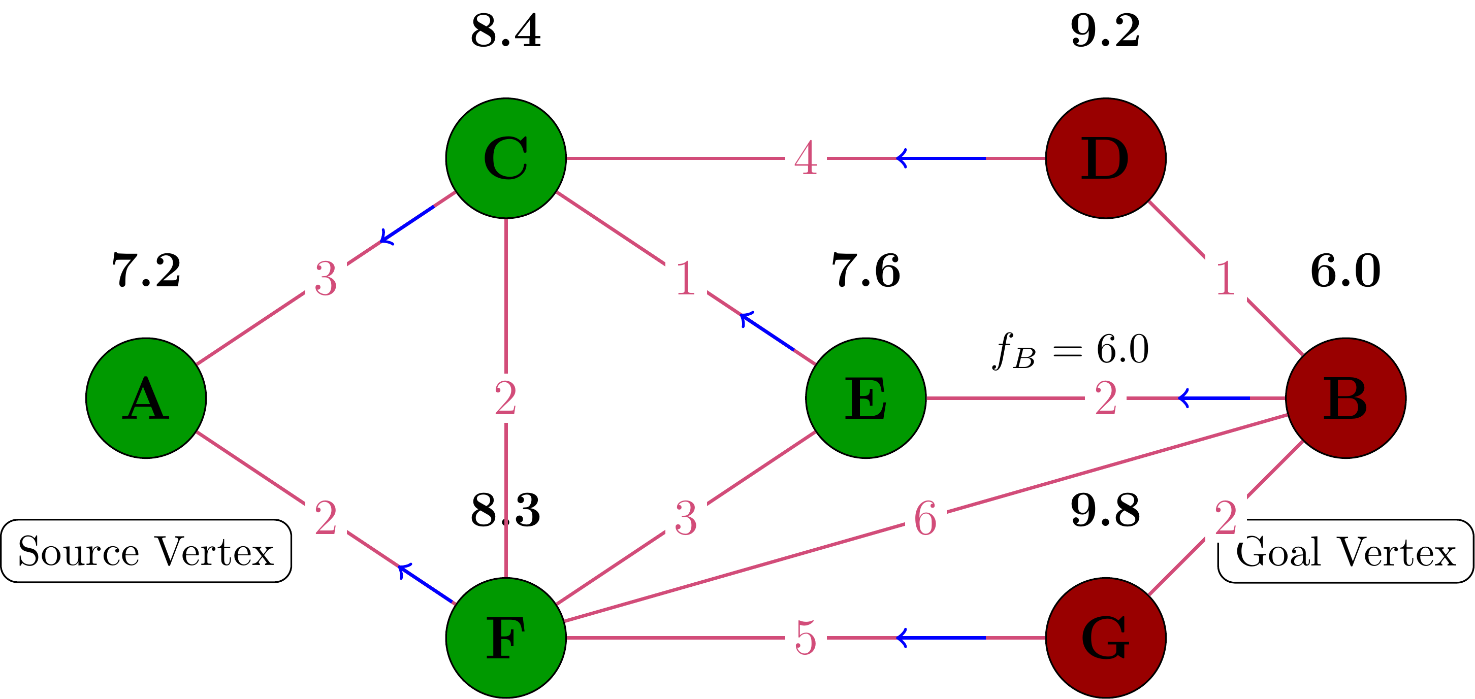
Vertex E has the lowest f-value, so we process it:

• Add E to the closed set (green)
• Update neighbor B with a better path (through E)
• B now has f-value = 7.0 (better than the previous 8.0)

Step 8: Finding Vertex B (Second Time)

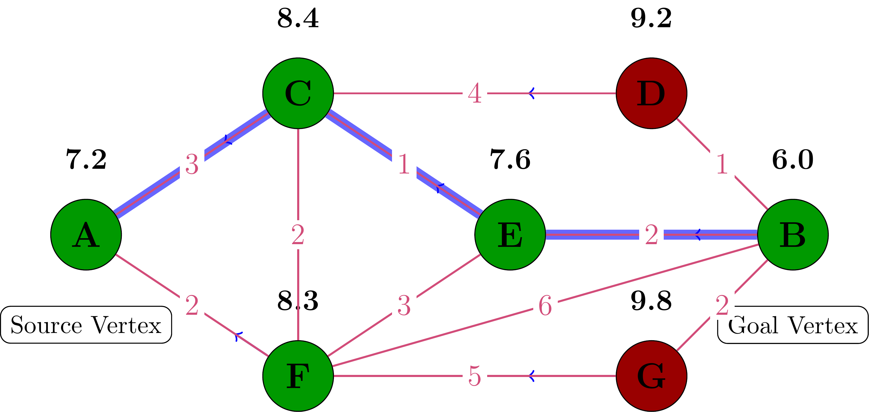
Vertex B has the lowest f-value (7.0), so we process it:

• Add B to the closed set (green)
• Since B is our goal vertex, we’ve found the shortest path!

Implementation Details

For a full Python implementation of A*, see my A* Implementation on Github.

References

Hart, P. E., Nilsson, N. J., & Raphael, B. (1968). A Formal Basis for the Heuristic Determination of Minimum Cost Paths. IEEE Transactions on Systems Science and Cybernetics, 4(2), 100-107. More references to be added…